Excel FILTER, SORT, UNIQUE, GROUPBY: Live Reports, No Copy

The video for this lab is in Hindi; the formulas on screen are standard Excel.

Dynamic array formulas spill: one formula returns a whole range that resizes when the data changes. Lab 6 builds a live report from them, driven by a region and year selector. It needs Microsoft 365; GROUPBY and PIVOTBY need a current build.

Step 1: Lists that keep themselves up to date

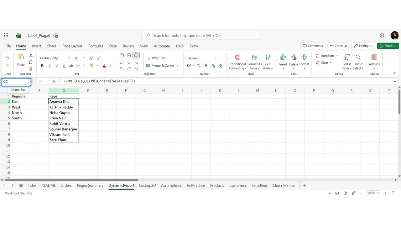
On a sheet named DynamicReport: =SORT(UNIQUE(tblOrders[Region])) and =SORT(UNIQUE(tblOrders[SalesRep])). Four regions and eight reps, each a spill range with a blue border. F2# refers to the whole spill range, however big it becomes.

Step 2: A selector driven by a spill range

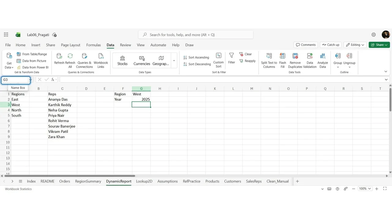
A Data Validation list with source =$D$2# gives a Region drop-down that updates when regions change, plus a Year drop-down.

Step 3: FILTER the orders

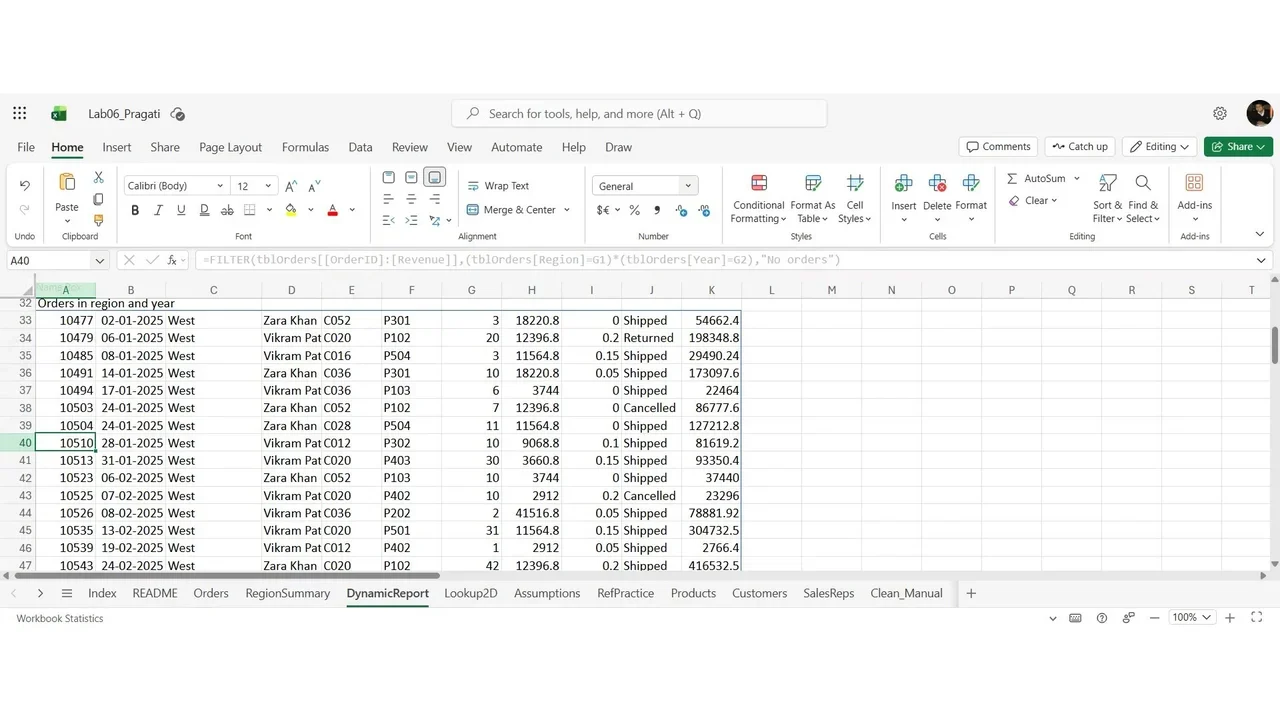
=FILTER(tblOrders,(tblOrders[Region]=B1)*(tblOrders[Year]=B2),"No orders")

Change the region and the result resizes. Type something inside the spill area and you see #SPILL!; delete it to fix.

Step 4: Top 10 with LET, SORTBY, TAKE and CHOOSECOLS

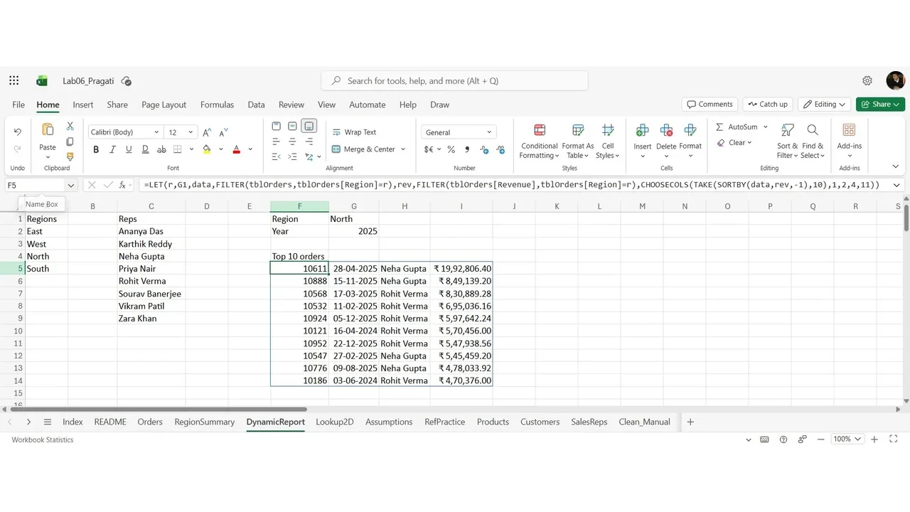
LET names each step so the formula reads like a recipe: filter by region and year, sort by revenue descending, take ten rows, and keep only the columns you need (XMATCH finds the Revenue column by name, so it survives column moves).

Step 5: A month list and stacked tables

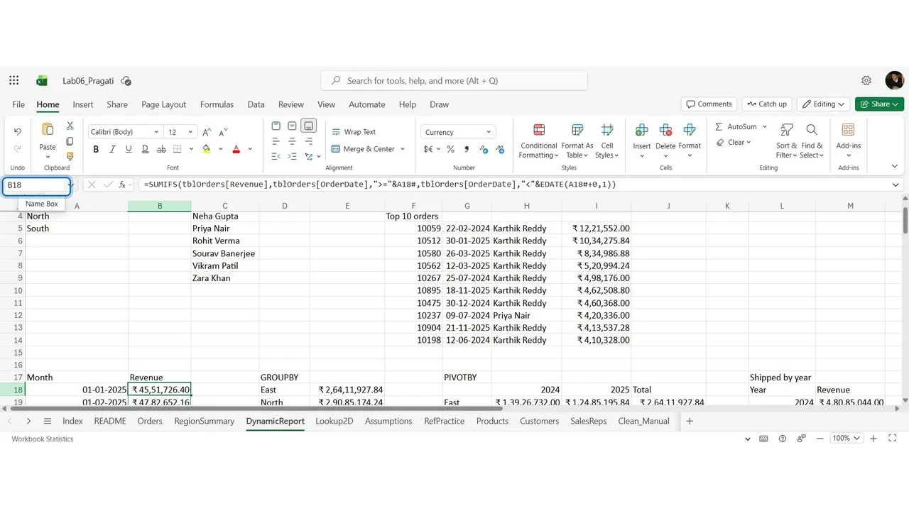
SEQUENCE builds twelve months; SUMIFS on that spill returns twelve revenues at once; VSTACK and HSTACK combine headers and data into one labelled table, ready for a chart.

Step 6: GROUPBY and PIVOTBY

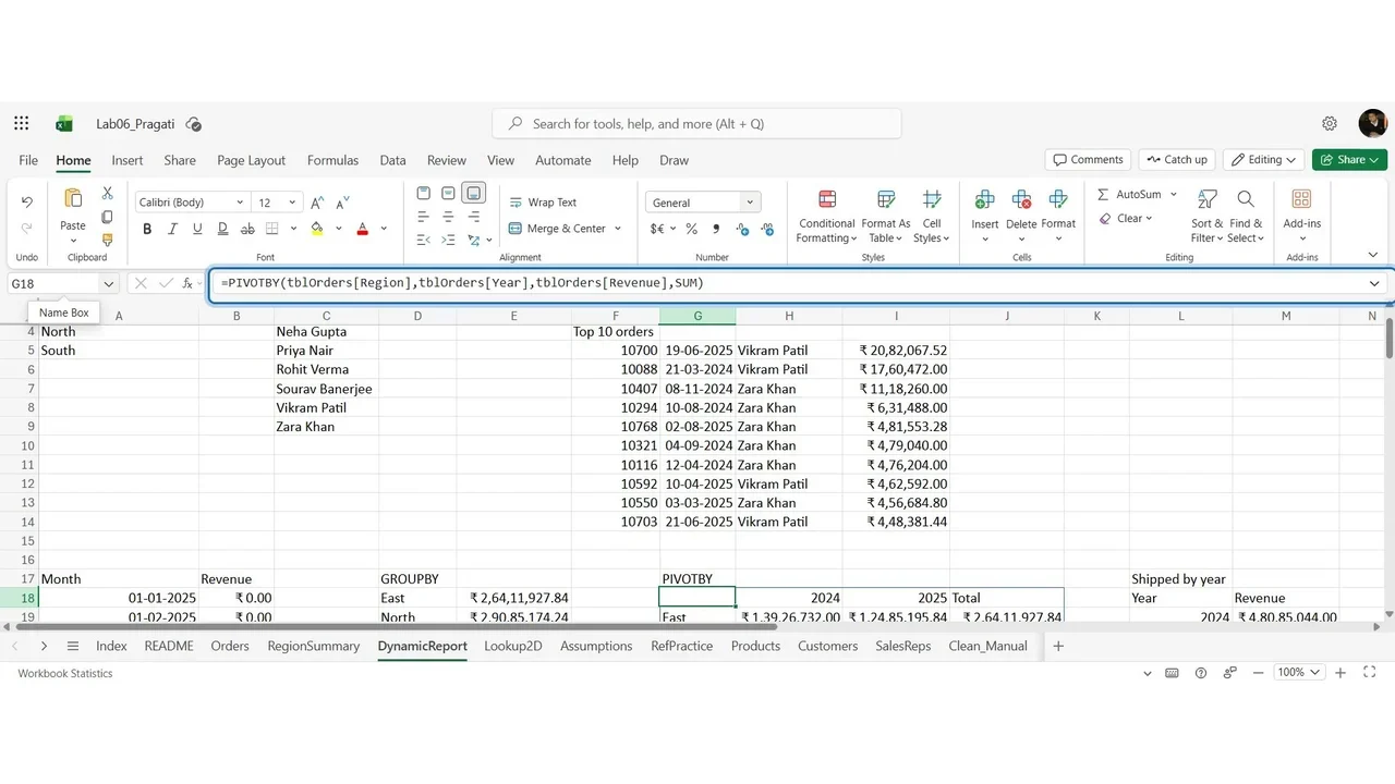
=GROUPBY(tblOrders[Region],tblOrders[Revenue],SUM) and =PIVOTBY(tblOrders[Region],tblOrders[Year],tblOrders[Revenue],SUM): a full region × year summary from one formula.

How you know it worked

Change the Region or Year drop-down and every spill range updates, with no #SPILL! or #CALC! errors. Compare the GROUPBY totals with your earlier region summary to confirm they agree.