Why VLOOKUP Breaks and XLOOKUP Doesn't, With Examples

The video for this lab is in Hindi; the formulas on screen are standard Excel.

Lookups connect your order table to products, customers and budgets. Lab 4 compares the three main approaches and then solves the harder cases: missing values, two-way lookups, several criteria and approximate matches.

Step 1: Three lookups, side by side

Add three columns to tblOrders and fill them three ways:

=VLOOKUP([@ProductID],tblProducts,2,FALSE)
=INDEX(tblProducts[ProductName],MATCH([@ProductID],tblProducts[ProductID],0))
=XLOOKUP([@ProductID],tblProducts[ProductID],tblProducts[ProductName])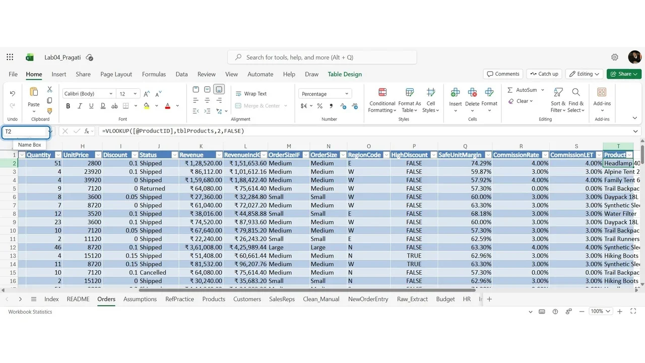

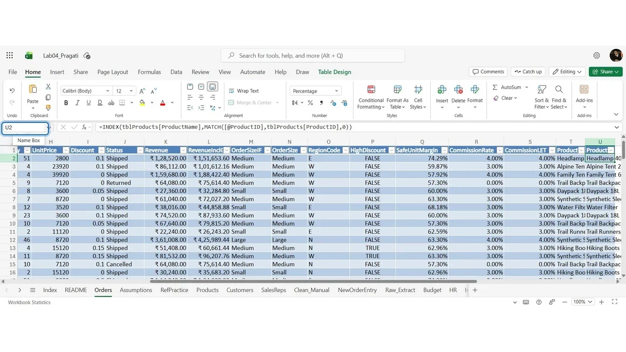
Now break VLOOKUP on purpose: insert a column in Products. VLOOKUP returns the wrong column, because it relies on a column number. INDEX/MATCH and XLOOKUP reference the column itself, so they survive structural changes. Keep XLOOKUP.

Step 2: Enrich the fact table

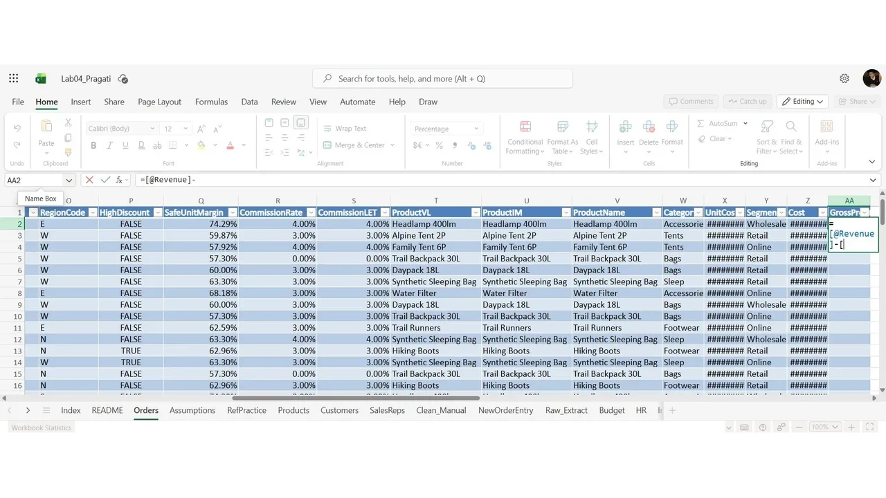
The same XLOOKUP pattern adds Category and Segment; then Cost = Quantity × UnitCost and GrossProfit = Revenue − Cost. Every order now carries what reports need.

Step 3: Missing values

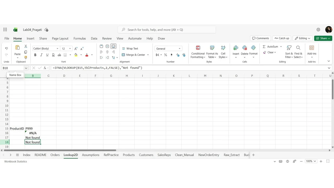
=XLOOKUP(A2,tblProducts[ProductID],tblProducts[ProductName],"Not found") returns Not found for an unknown ID like P999. The INDEX/MATCH equivalent needs IFNA(..., "Not found").

Step 4: Two-way lookup

Build a region × category grid with SUMIFS, then pick one cell by name:

=INDEX($B$7:$G$10, XMATCH(I6,$A$7:$A$10), XMATCH(I7,$B$6:$G$6))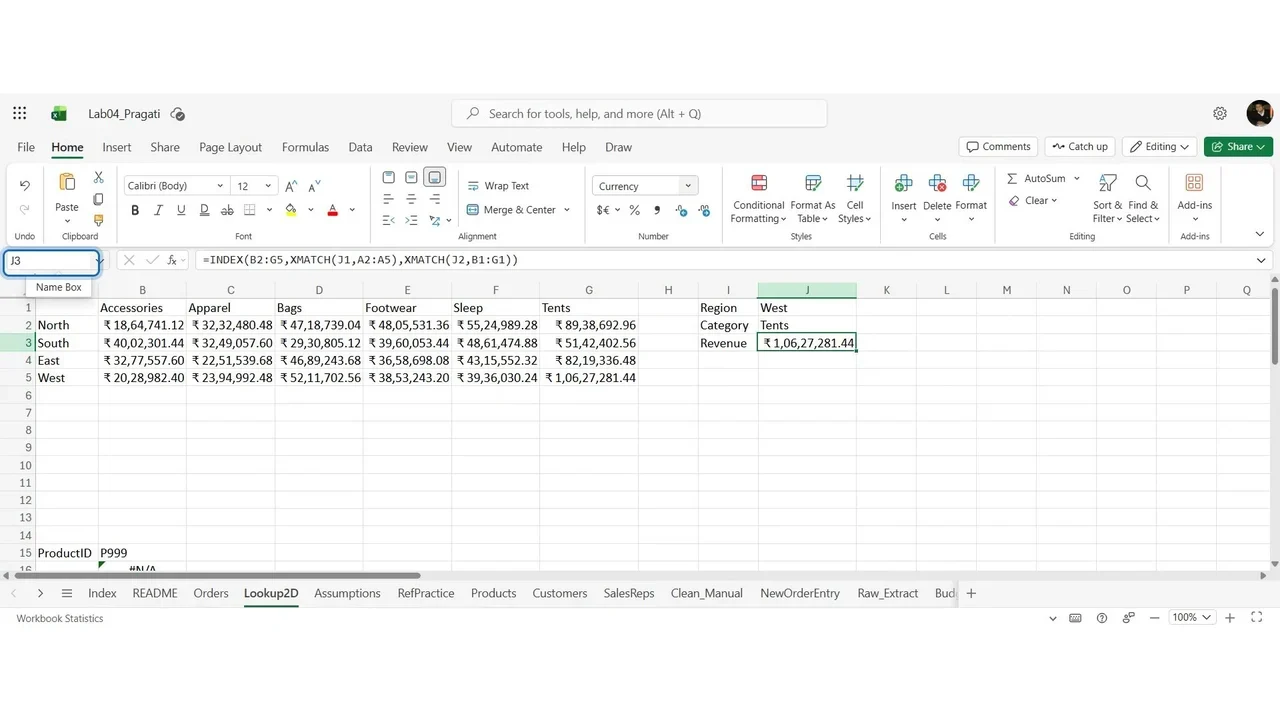

Step 5: Several criteria

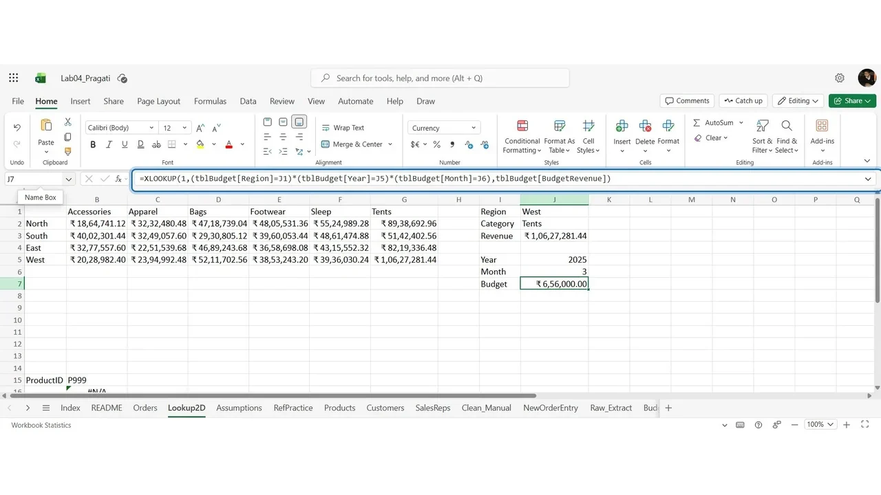
Find the budget for a region, year and month in one formula:

=XLOOKUP(1,(tblBudget[Region]=K6)*(tblBudget[Year]=K7)*(tblBudget[Month]=K8),
         tblBudget[BudgetRevenue],"No budget")

Each comparison returns TRUE/FALSE; multiplying them gives 1 only where all are true, and XLOOKUP finds that 1.

Step 6: Approximate match for commission tiers

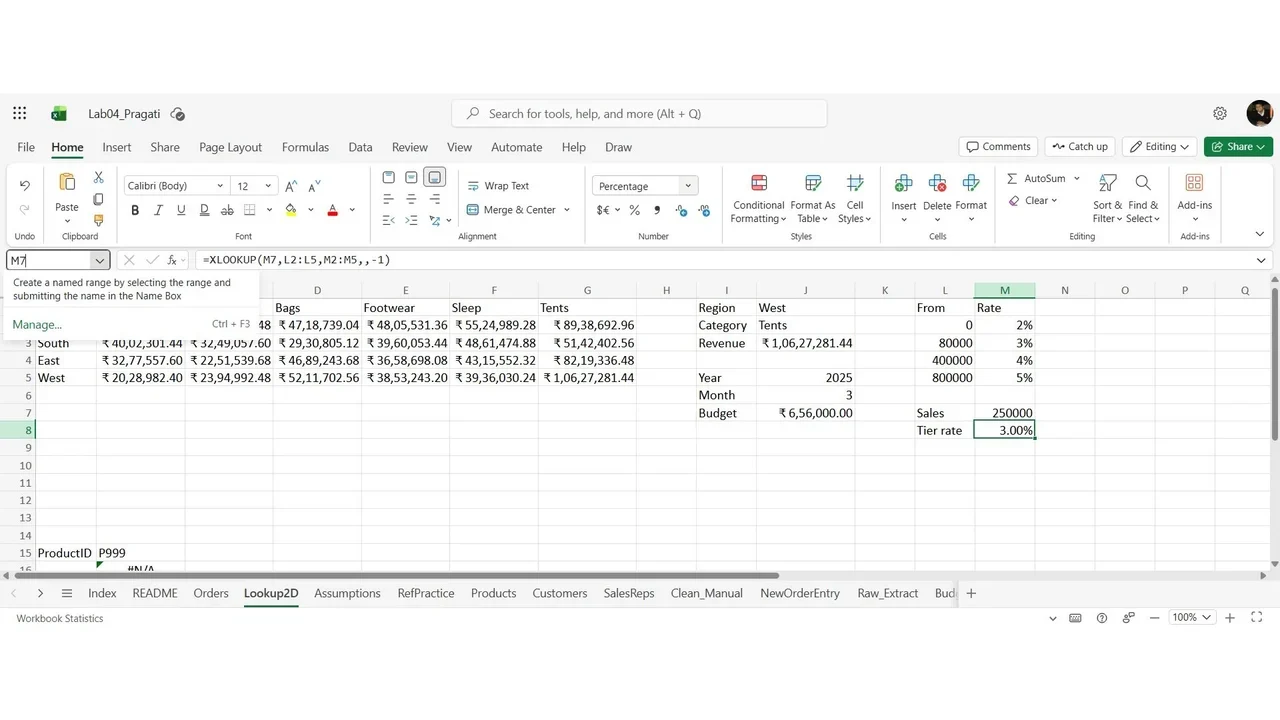
With a tier table (from-amount and rate), =XLOOKUP(M13,M7:M10,N7:N10,,-1) returns the rate for any sales amount. Match mode −1 means exact match, or the next smaller item. The classic equivalent is VLOOKUP with TRUE, which needs the table sorted ascending.

How you know it worked

Total gross profit is calculated with no #N/A anywhere in the orders table, and every special lookup returns the expected value when you change its inputs.